3.5.1.3 (Controlled) Random waveforms
You could also record noise into an array and then read it out periodically - i.e., read the same thing out again and again (cf. Karplus-Strong). If you do this more than 20 times a second, you'll hear a pitch:
너는 어레이에 노이즈를 레코딩하고 그것을 주기적으로 읽어올 수 있다. 같은 걸 읽고 읽고, 만약 이것이 일초에 20번보다더 하게 되면, 너는 피치를 듣게된다.
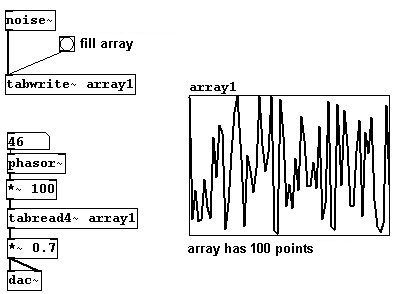
The spectrum of this sound is naturally somewhat unpredictable. Every time you fill the array with random numbers with the "noise~" object, you get a new wave with new characteristics.
But there is still somewhat of a system at work. You could, for example, interpolate all the clicks (large jumps in the waveform) to achieve a smoother resultant waveform. Let's generate random points using linear interpolation ("Uzi" (Pd-extended) generates the number of bangs specified in its argument and sends them as fast as possible):
이 소리의 스펙트럼은 자연적으로 다소 예측이 안된다. 너가 어레이를 노이즈 오브젝트에 랜덤 숫자들로 채울때마다 너는 새로운 캐릭터의 웨이브를 얻게된다. 하지만어쨌거나 작동하는데 체계는 있다. 예를 들면, 모든 클릭들을 내삽(평균)할 수 있는 데 그를 통해 결과적으로 더 부드러은 웨이브폼이 발생한다. 선적인 내삽으로 랜덤포인트들을 발생시키자. (uzi가 특정 변수에 뱅들의 값을 발생히키고 최대한 빨리 그들을 보낸다. )
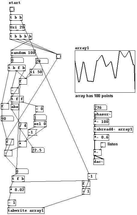
In this example, four points are always used for interpolations.
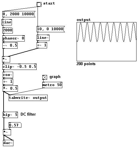
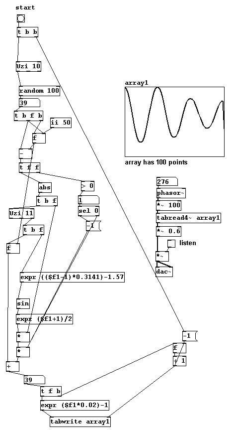
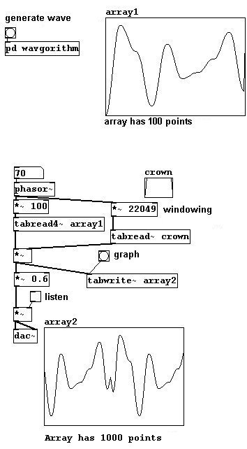
The result will be even softer if you use a sinusoid interpolation instead of a linear one. Here, ten points are used for interpolations:
이 예에서 네 점이 항상 내삽(평균값)을 위해 사용된다. 그 결과는 너가 선적인 것 대신 사인곡선 평균을 사용했을때 더 부드러워 질꺼다. 여기 10지점이 평균내는데 사용되었다.
patches/3-5-1-3-wavgorithm+sin.pd
Now the connection from the end of the period to its beginning has to be interpolated as well. We'll use a windowing for this and program the calculation in a subpatch.
이제 끝에서부터 그것의 시작까지 연결은 마찬가지로 평균(내삽)되어야 한다. 우리는 서브패치로 계산하는 프로그램을 만들어서 창으로 사용하곤 한다
patches/3-5-1-3-wavgorithm+sin+fenster.pd
This way, the membrane is at 0 at the beginning and end of each period. The result could be even smoother if it were "windowed" with the Hanning window (3.9.4.1).
In addition, transfer functions using known waveforms - e.g., a square wave, which would intensify the odd partials - are also possible.
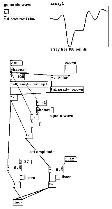
And so on. In these last few examples, the wave has to be created on the control level; in contrast to the first examples that used transfer functions, we cannot change these "live".
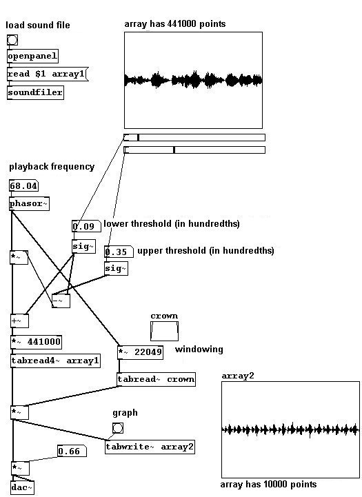
3.5.1.4 Wave stealing
A final technique that might be considered wave-shaping synthesis is "wave-stealing". This involves taking a small section of known pieces of music...
patches/3-5-1-4-wavestealing.pd
3.5.2 Applications
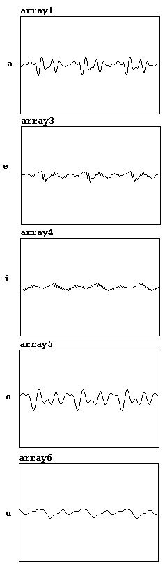
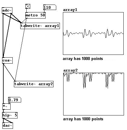
3.5.2.1 Singing waveforms
With the following patch, it is possible to record waveforms with a microphone to sing waveforms.
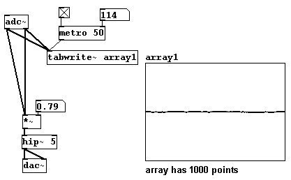
The vowels (German pronunciation) look something like this:
3.5.2.2 Transfers
And this input signal could naturally also be sent through a transfer function:
3.5.2.3 Even / odd partials
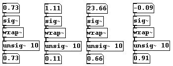
You can also divide a sawtooth wave into even and odd partials. To accomplish this, you'll need to use "wrap~". It calculates the difference between the input number and the nearest integer below it (the absolute value is taken, so that the result is always positive). A few short examples:
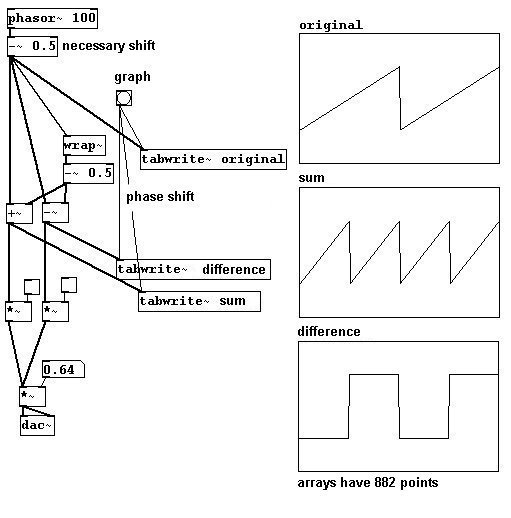
And now for the sawtooth division: the "wrap~" object is used to phase shift the sawtooth wave; this is then added to and subtracted from the original signal, resulting in a sawtooth wave with twice the frequency and a square wave.
patches/3-5-2-3-even-odd-partials.pd
3.5.2.4 More exercises
a) Create a wave that changes constantly.
b) Create a patch in which the interpolation and array points used for (controlled) random waveforms are variable in number.
3.5.3 Appendix
3.5.3.1 Foldover
At this point, a particularly thorny problem in digital sound processing must be addressed: foldover. Let's first examine this situation:
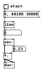
What happens? After 22050 Hz, the direction changes until it reaches 44100 Hz, at which point you get a pitch with a frequency of 0 Hz (after this, the pitch would go up again). The reason for this is that a sample rate with of 44100 Hz can produce a wave of 22050 Hz maximum (cf.3.1.1.3.1). Moreover, there are some typical reading errors. Let's take a look at three waves with different frequencies: the top has a frequency of 11025 Hz, the middle 22050, and the bottom somewhat more than 22050. The markings stand for reference points (for the samples), which have a constant speed of 44100 per second.
deh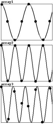
Each period in a wave with 11025 Hz can be represented with four points (of course, the characteristic sine wave shape is lost). 22050 Hz is the highest frequency that can be correctly represented, since Nyquist's Theorem requires at least two points per period. Errors will occur with frequencies higher than this; not every period will be captured and the points of measurement will actually record a lower frequency instead of a higher one.
The problem is much more pronounced for waveforms that exhibit overtones, e.g., with a pulse:
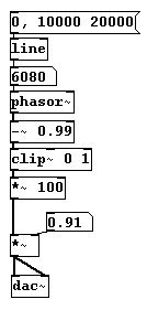
Here the effect can be noticed much earlier: after 700 Hz some overtones are inaccurately captured. This is because the pulse waveform practically consists of just a single line, which is quickly 'missed'. A solution to this problem is to begin with a pulse waveform, but to broaden the wave as the frequency increases, so that you end up with a sine wave at the end: